Will the Stock Market Crash?

Will the stock market go down in the next six months? The general answer: probably not. The correct answer: sometimes, in unique situations, you have better odds of making money being short equities instead of long equities.

The market goes from undervalued to overvalued on a regular basis. Fortunately, there are tools for assessing how to utilize thoughtful systematic methods to best gauge where the market is going. In this piece, we will discuss a framework for assessing the relative attractiveness of the U.S. stock market in the context of a widely accepted equity valuation model - The Dividend Discount Model - and what factors can contribute to the expected returns of equities.

Due to the tendency of the stock market to increase in value, predicting down periods is a complex, nuanced process that can only be discerned through the weight of the evidence from many orthogonal concepts. One such piece of evidence might be real estate activity in Manhattan. In 2018 Q2, Manhattan’s residential real estate market experienced a market-wide decrease in the number of sales, falling 16.6% to 2,629 units, which is the lowest second-quarter sales since 2009¹. This drop was the third consecutive quarterly decrease. Listing inventory rose 10.7% year-over-year to 6,985 active listings, while the listing discount grew to 4.1% over the previous quarter¹.

A Macro trader might weave discrete pieces of information like these into an anecdotal story to short the stock market. There are clearly tipping points where several inputs can signal tops in the equity market, but it is not a simple matter to short the stock market without a mosaic of inputs. Would you short the stock market with the Manhattan real estate information alone? Probably not; but add other corroborating evidence that might suggest the end of an expansion period - such as spiking real estate prices, cyclically high corporate profit margins, or slowing corporate sales growth - and maybe you could think about shorting the stock market.

For a Systematic Macro trader, a single fundamental observation or an isolated overbought indicator cannot produce a short. There are cycles in the market and the frequencies of these cycles are changing. A statistical time series study can be misleading when attempting to short the market: the more time-dependent your study, the more likely it will miss important price action. The fact that a market is overextended on a fixed lookback of performance likely does not independently hold value, as the best forecast for tomorrow is for a market to continue its current trend. For a sell-off to be reliably predicted by a systematic macro trader’s inputs, the overall state of the economy must shift as a result of substantial changes in macroeconomic releases.

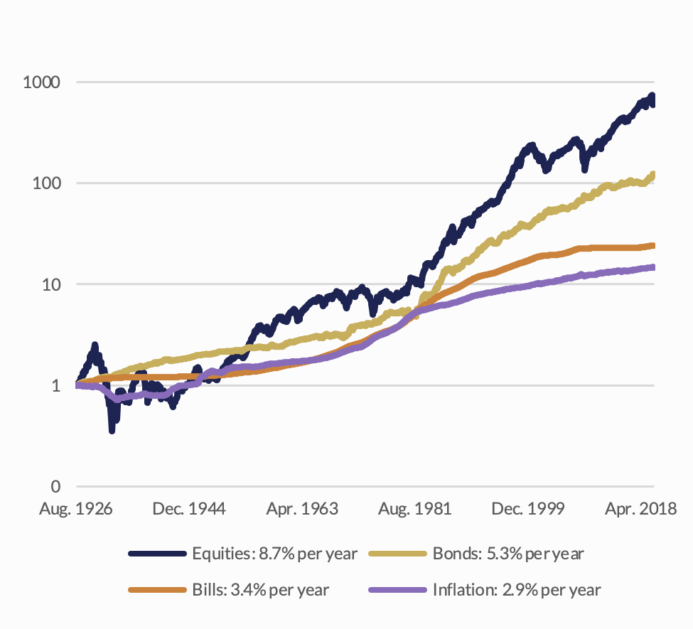
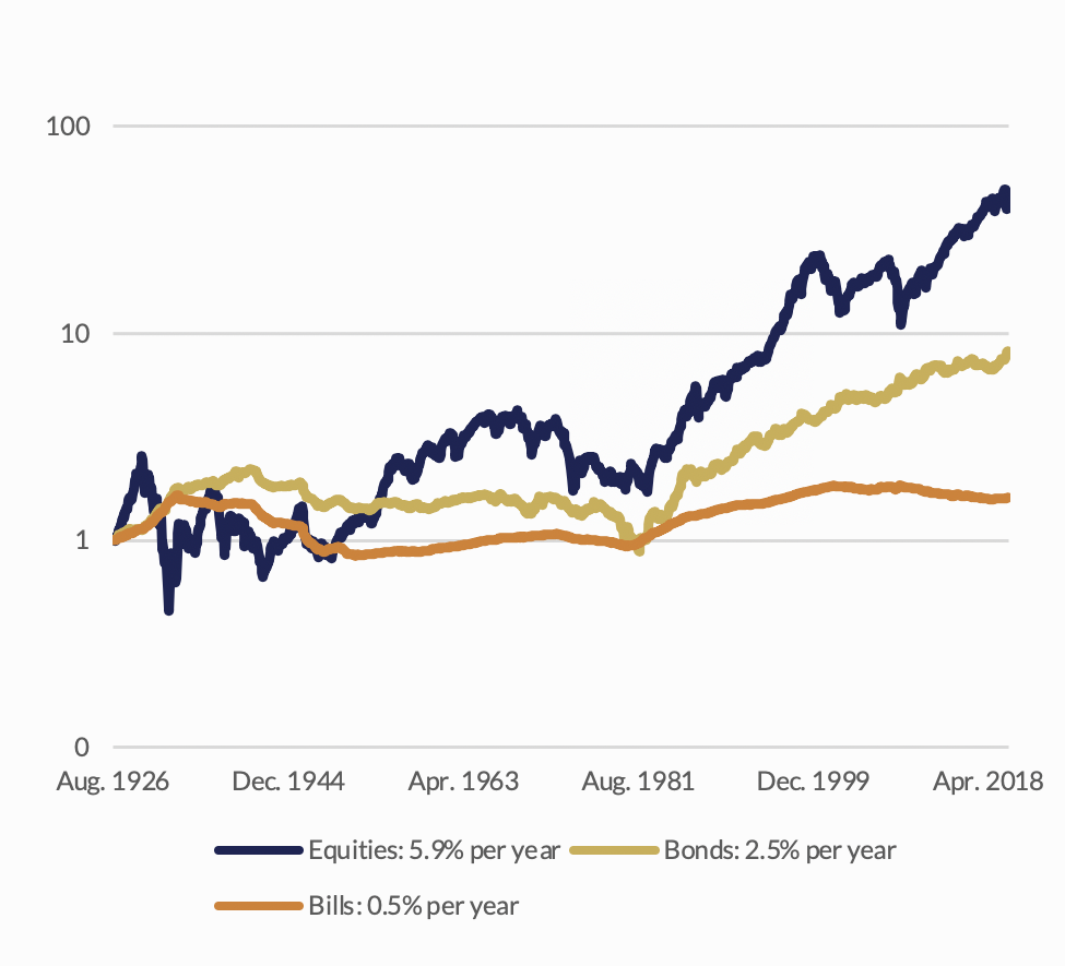
Historically, U.S. Equities have been the highest performing asset class, delivering approximately 9.6% nominal and 6.5% real returns; they have outperformed Short-Term and Long-Term US Treasury Bills by 6% and 4.5%, respectively². The two graphs below compare the US asset classes in both nominal and real terms from 1900 to 2017^2,3.

Cumulative Returns on U.S. Asset Classes, 1926-2020

Nominal Terms

Real Terms

From a bird’s eye view, the stock market is more likely to go up than down. The S&P 500 has had the following percentage of positive returns over the following timeframes⁴:

Given this fact, you need a robust approach to bet against the house. The Dividend Discount Model (DDM), also known as the Dividend Growth Model or Gordon Growth Model, provides a framework on how to conceptualize and calculate equity valuations. Essentially, DDM values a stock using the following inputs: the stock’s dividends, the growth rate of the dividends, and the market risk premium due to interest rates, idiosyncratic risks, market sentiment, etc.

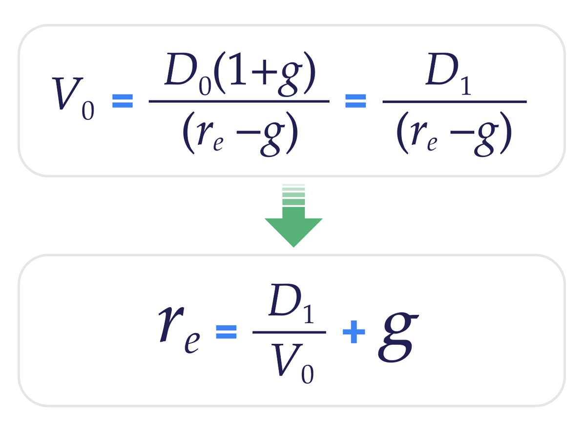
V₀Value of the Stock

D₀Dividends Today

D₁Dividends @ t+1

r_eMarket Risk Premium

gDividend Growth Rate

D₁/V₀Dividend Yield

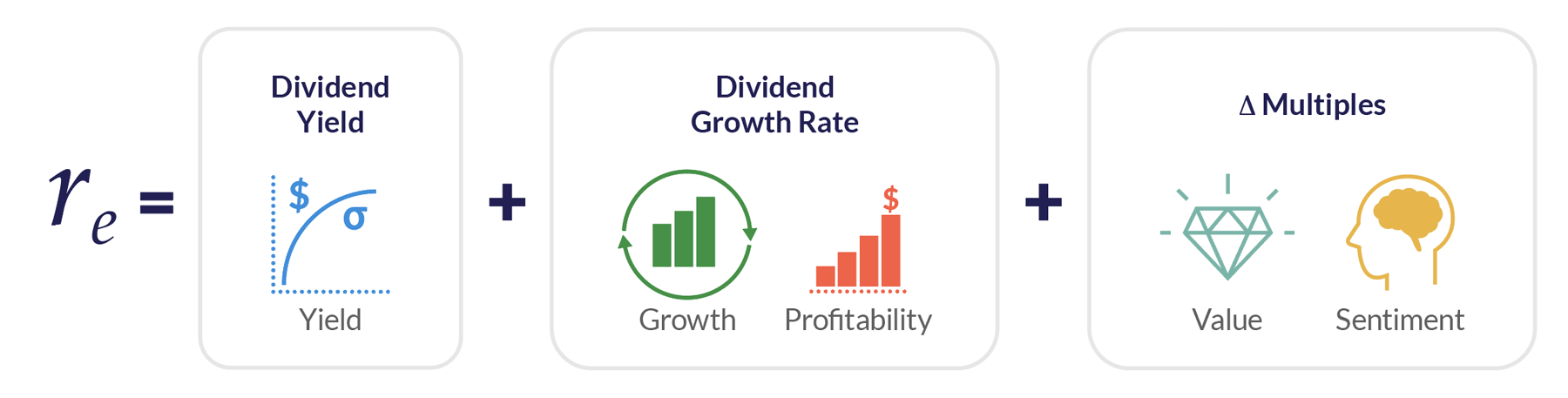
The Dividend Discount Model is based on deriving an estimation of price for a single point in time. In order to perform a forward-looking estimation, we must take into account the variability in multiples. By rearranging the Dividend Discount Model equation as above and adding the effect of changing multiples, we get an extension of DDM to forecast returns of the stock market. The three terms of this equation are estimated using a 5-factor framework that we believe covers most of the reasons why stocks are attractive or unattractive; these are all derivations of the factors and trading models used by our Systematic Global Macro program:

The Dividend Discount Model (and our extension thereof) is robust, but its primary weakness lies in the uncertainty of the inputs. Small changes in the inputs can result in large changes in the expected value. This uncertainty is mitigated to a certain extent by our systematic approach to measuring each input, but there is still a daunting imperative to provide an accurate and timely measurement.

This framework gives a daily read on the attractiveness of US stocks and what percent we would choose to be invested. The answer the framework gives to the question, will the stock market crash, depends to a great degree on the time in history when the question is asked.

Estimating Dividend Discount Model Inputs

Estimating Dividend Yield

Dividend yield – or better yet, total yield – is the easiest input of the framework to estimate with relative confidence. Dividend yield is what most carry strategies aim to capture; therefore, estimating dividends is usually an appropriate start to estimating expected returns. Historically, dividend yield has been an effective stock market predictor⁵; however, there are important statistical issues related to its high degree of autocorrelation when used in this manner⁶.

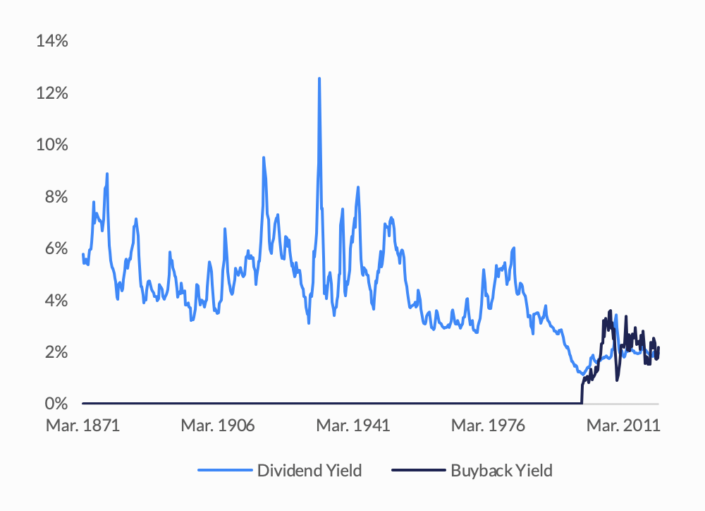
Since the mid-1990s, dividend yield has decreased because many companies have transitioned the capital previously used for dividends to stock buybacks for tax purposes, creating a structural break. As shown in the graph below, the size of buybacks is currently larger than the size of dividends. Thus, ignoring the buyback effect negatively biases the expected return.

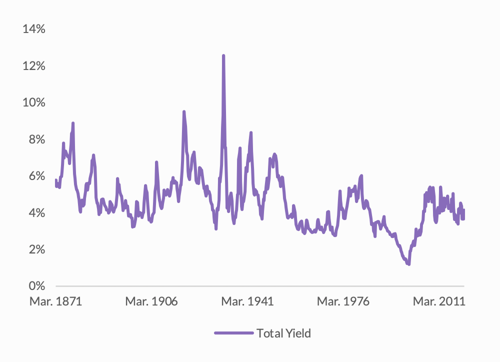
Dividend Yield & Buyback Yield, 1871-2020

Dividend Yield & Buyback Yield

Total Yield

Arnott and Bernstein argue that the return from buybacks at the aggregate stock market (such as the Wilshire 5000) is smaller than the net stock issuance, including issuance for both M&A and IPOs. However, when working with a subset of stocks (such as the S&P 500), the effect of new issuances is small because there are only secondary offerings, and each stock departure from the subset is quickly filled with another stock⁷.

Studies show that companies with buybacks outperform the market; therefore, adjusting the dividend yield to include the buyback effect improves the DDM’s forecasting power⁸. The above graphs outline this effect; the left graph shows Dividend Yield and Buyback Yield separately, and the right shows the two yields combined as Total Yield⁹.

Our estimation of this term of the equation is derived from the Yield factor of the 12 Box Framework, which measures the absolute expected real yield adjusted for volatility. Assessing the real, expected, and risk-adjusted yield of equities provides a good read of their attractiveness over a medium-long term horizon (~30-60 days).

Estimating Dividend Growth

Growth is the second hardest input to estimate and can be forecasted using a top-down or bottom-up approach. A top-down approach uses the broad economy (i.e. GDP per capita growth rate) as a proxy but often lacks practical implementation. A bottom-up approach aggregates analysts’ firm-level expectations but typically suffers from their individual biases. We use both types for our estimation of growth.

Historically, during periods more than 10 years, earnings growth per share for U.S. stocks has been in line with U.S. GDP growth per capita at around 2%¹⁰. Forecasting and nowcasting economic growth are at the center of most macroeconomic models due to the stickiness of economic growth¹¹, including our own.

GDP growth has almost no actionable predictive power because of its lag in reporting. In order to estimate growth reliably, we use actual weekly and monthly macroeconomic data releases. The growth models from our Systematic Macro trading program capture changes in economic growth expectations by distilling macroeconomic releases into an actionable read that evaluates Equities over a somewhat short-term horizon (~10 days).

The bottom-up component of our estimation of growth analyzes aggregate S&P 500 earnings with their growth and stability over the last 3 and 12 months. The consistency, sustainability, and growth of profits is what ultimately drives equity returns. This read is another medium-/long-term read: ~50-100 days. However, it does little to explain the reasons that earnings multiples contract and expand over time.

Estimating Multiples

Multiples are the hardest input to forecast over the short-term. Long-term forecasting is slightly easier as a result of their mean-reverting tendency. Commonly, expected return estimations focus only on yield and growth, ignoring multiples entirely. Multiples are able to drift higher as a result of sustained optimism about the future of the market. Low multiples persist as a result of market cynicism.

In other words, multiples capture and reflect investors’ risk appetite, which is driven and measured by a variety of factors: namely market sentiment, geopolitical risk, inflation, interest rates, regulatory risk, and transaction costs. Most value approaches are based on mean reversion of some form of multiples (price-to-earnings, price-to-book, and price-to-cash flow) over long time frames, defined as 5-10 years or more.

Cyclically Adjusted Price-to-Earnings (CAPE) Ratio

U.S. Equities, 1931-2020¹²

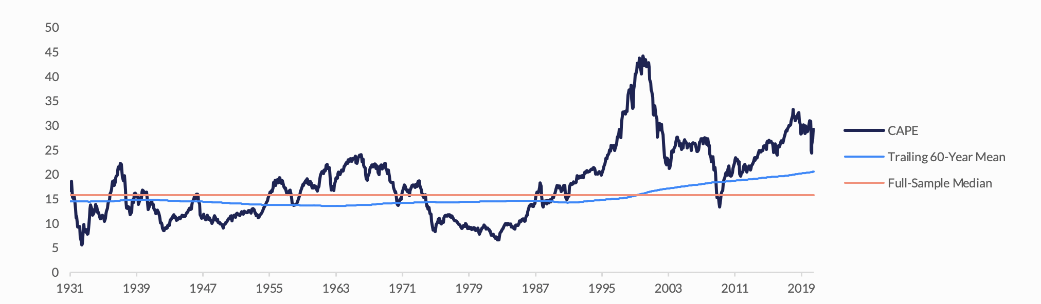
As the graph illustrates, the limitation of this approach is that multiples have been drifting higher over the last 50 years compared to the previous 50 years due to lower global risks: rising risk appetite, waning inflation uncertainty, historically low interest rates, and higher costs.

This upward drift, or increasing mean, in multiples makes mean reversion analysis challenging, resulting in a poor out-of-sample performance for directional equity valuation models. Value approaches have been more successful when applied on a relative basis within asset classes, across countries¹³. The benefit of the relative value approach lies in the use of the more stable, cross-sectional mean versus the more volatile, time-series mean. Value is a simple metric of volatility-adjusted P/E relative to the last 5 years. On its own, value offers very little insight due to its low frequency (~40-75 days) and the danger of selling an overvalued condition.

Purely price-based trading models are also implemented to capture the downstream impacts of transitory changes in market sentiment that cause multiples to wax and wane. These models try to take advantage of short-term (less than one month) and medium-term (up to one year) patterns in sentiment by employing statistical price analysis. The patterns captured are usually short-term mean reversion and medium-term trend-following because of investors’ tendency to overreact to new information in the short-term and slowly digest the information in the medium-term. The fluctuating ability of market participants to contemporaneously respond to incremental information indicates to us that a fundamental approach is more reliable.

In order to gauge the effect of this trend on estimated equity returns, a macro view must measure market sentiment in some way. Our approach to estimating sentiment is centered on crucial cognitive biases of a variety of market participants. We utilize our equity-specific signals from our sentiment models within our Systematic Macro portfolio. There are regularly short-term threats to the market where investor sentiment turns particularly positive or negative. This is a very useful tool in modulating equity exposure in a more tactical ( <10 days) fashion.

Changes in the growth of multiples due to market sentiment create the majority of the opportunity when timing investments in the stock market. Independent of earnings reports, the market can turn bearish solely due to negative market sentiment; investors simply do not “like” stocks as much in the future as they do in the present. This negative market sentiment can be created by a number of different environments: fear of taxes, fear of rising inflation, perceived decrease in economic activity, war, and political uncertainty, to name a few.

So...will the stock market crash?

Given that the market goes up 71% of the time in a 6-month window, it is a much better bet that the market will go up. The better way to frame the question is: Does the weight of the evidence warrant being short the market? We can use our extension of the Dividend Discount Model - estimating growth in earnings and estimating growth in multiples - to answer this question.

By definition, earnings have a very real and positive bias. Public companies make money because they sell products that meet consumer demands for a profit. To bet against this assumes you believe companies will lose money, cease dividend payments, and shrink their balance sheets. This negative earnings scenario can be created by reduced revenue/top-line sales, increased input cost, or a combination of both. It is virtually impossible to bet on a catastrophic economy that creates negative profits. In any 6-month window since 1993, S&P 500 companies have reported positive absolute trailing 12-month earnings per share 86% of the time¹⁴.

Aside from being positive from the absolute perspective, can we determine if earnings will actually go down in the next 6 months? Since 1990, earnings have risen 61% of the time in any 6-month window¹⁴. Therefore, a decrease in earnings is possible to forecast, yet difficult, at only 39% of the time. In addition, forecasting and capitalizing on this negative change requires a high amount of accuracy in estimating economic inputs, such as GDP growth and inflation, as well as a high amount of accuracy in deciding which stocks are directly affected.

The question, will the stock market go up or down, can be conceptualized in the following way:

Imagine someone trying to escape from a Mama Grizzly via hot air balloon. Growth and yield act as the engine powering the balloon, fueling the upward movement. Without positive yields and growing underlying economies, stocks can’t hope to get off the ground. Profitability, value, and sentiment can all be thought of as ballasts that may or may not inhibit the potential of the stock market. With prevailing negative sentiment, you are effectively tossing a 200-pound anvil out of the basket tied to your foot. With solid value, you’re cutting the rope to release a ballast, allowing the opportunity provided by growth and yield to send the balloon up.

So, will the ballasts outweigh the power of the engine? Can you rationally short the stock market in the next 6 months? The following concepts might help:

1. Multiples mean revert; high multiples will turn into low multiples. The question to answer is: Will multiples revert faster than earnings will rise? In other words, “cheap” and “expensive” are real but difficult to time.
2. Cyclically high-profit margins also mean revert, typically correlated to overall multiples cycles.
3. Economic cycles are real with varying frequencies and positive serial correlation. This behavior can help predict changing multiples with some accuracy.
4. Prices also tend to follow a trend. Therefore, economic cycle data presents itself in price movements: a downtrend in price can help predict future down prices.
5. General market sentiment and investor fear are real and can change quickly. There is a benefit to measuring and anticipating a rising fear level or reduction in risk appetite, as this can lead to lower multiples.

All these tools and concepts have small marginal utility and make it difficult to make bold 6-month predictions. They can, however, be very helpful in making small, incremental, cumulative bets on a down market - in 1-3-week windows - that can sequentially cascade into an accurate 6-month view of the market.

References

1. Elliman Report, Q2 2018 Manhattan Sales.
2. Dimson E., Marsh P., Staunton M., 2018, “Credit Suisse Global Investment Returns Yearbook 2018”.
3. Dimson E., Marsh P., Staunton M., 2002, “Triumph of Optimists.” Princeton University Press and subsequent research.
4. Bloomberg.
5. Campbell, J. 1991, “A Variance Decomposition for Stock Returns”, Economic Journal, 101, 157-179. Cochrane, J. H, Hansen L. P. 1992, “Asset Pricing Explorations for Macroeconomics”, NBER Macroeconomics Annual 1992, Volume 7, Blanchard and Fischer.
6. Goetzmann, W. N., P. Jorion. 1993. Testing the predictive power of dividend yields. J. Finance 48(2) 663–679.
7. Arnott, R. D. ,Bernstein, P. L., 2002, What Risk Premium is “Normal”?, Financial Analysts Journal, 58:2, 64-85.
8. Boudoukh, Jacob, Roni Michaely, Matthew Richardson, and Michael R. Roberts. 2007. “On the Importance of Measuring Payout Yield: Implications for Empirical Asset Pricing.” The Journal of Finance, 62: 877–915.
9. Philip U. Straehl & Roger G. Ibbotson (2016) The Long-Run Drivers of Stock Returns: Total Payouts and the Real Economy.
10. Arnott and Bernstein, 2002. Ibbotson, Roger G., and Peng Chen. 2003. “Long-Run Stock Returns: Participating in the Real Economy.” Financial Analysts Journal, vol. 59, no. 1 (January/February):00–00.
11. Philip U. Straehl & Roger G. Ibbotson (2016) The Long-Run Drivers of Stock Returns: Total Payouts and the Real Economy.
12. Asness et al., 2017; Robert Shiller’s Data Library.
13. Asness et al., Value and Momentum Everywhere.
14. Bloomberg, Diluted Earnings per Share.